

Accurate experimental band gap predictions with multifidelity correction learning


Abstract
To improve the precision of machine-learning predictions, we investigate various techniques that combine multiple quality sources for the same property. In particular, focusing on the electronic band gap, we aim at having the lowest error by taking advantage of all available experimental measurements and density-functional theory calculations. We show that learning about the difference between high- and low-quality values, considered a correction, significantly improves the results compared to learning on the sole high-quality experimental data. As a preliminary step, we also introduce an extension of the MODNet model, which consists of using a genetic algorithm for hyperparameter optimization. Thanks to this, MODNet is shown to achieve excellent performance on the Matbench test suite.
Keywords
INTRODUCTION
The discovery of functional materials is the origin of many technological advances, from batteries to optoelectronic devices[1]. Given the extent of the compounds' space, it is essential to achieve fast and reliable screening to identify new and interesting candidates. In this framework, thanks to the growing number of available experimental and theoretical data[2-4], machine learning (ML) has recently emerged as an extremely useful tool[5-7]. However, obtaining reliable ML models typically requires large and high-accuracy datasets. Unfortunately, there is often an inverse correlation between quantity and quality. Large datasets are, in many cases, theoretical ones, such as those based on cheap density-functional theory (DFT) functionals, while high-accuracy experimental datasets usually have a rather small size. For instance, if one considers the electronic band gap (i.e., without excitonic effects), the Materials Project[8] contains
More generally, material properties are often bundled with different degrees of accuracy. The most straightforward case is a dataset gathering both experimental and DFT results, but it is not uncommon at all to see a dataset combining calculations computed with different exchange-correlation functionals such as PBE and the more accurate Heyd–Scuseria–Ernzerhof (HSE)[13].
For screening materials, one ideally wants to obtain the best estimate of the actual value (i.e., experimental) of the required property. This means that models should, in principle, only be built from scarce experimental data. In practice, it is, however, possible to gain knowledge from the larger but less qualitative datasets in order to improve predictions of the experimental quantity. This idea has already been investigated previously[14, 15]. Kauwe et al. [14] combined multiple learners, forming a so-called ensemble learning model, which was trained on experimental or DFT band gap data. The different predictions are then combined in a separate model, a meta-learner, predicting the final higher quality (i.e., experimental) data. Chen et al. [15] built a convolutional graph neural network based on MEGNet, where the fidelity of each sample is encoded through an embedding to form an additional state feature of the crystal. This method has the advantage of working on sets of compounds that can be very diverse, in the sense that all the compounds do not have to be present in each dataset (in contrast to Kauwe's method). However, given the complexity of the graph neural network, the errors are still slightly higher than with state-of-the-art methods relying on the smaller experimental dataset only[16].
Another popular strategy is to use transfer learning. In this approach, a neural network is first fitted on a large source dataset, followed by fine-tuning on a smaller target dataset. The network will transfer knowledge (embedded in the weights) from the source to the target task. This technique has successfully been applied in several studies, covering properties from Li-ion conductivity for solid electrolytes to steel microstructure segmentation[17-23]. To be effective, the source task should be closely related to the target task.
In this work, we compare different techniques that combine multiple quality sources for the same property in order to improve the accuracy of the predictions. The property of interest is the experimental band gap. Various studies have tackled the band gap problem (experimental and simulated), from composition or structure-specific tasks to more general approaches[10, 18, 24-29], with only more recently efforts on a multi-fidelity approach[14, 15]. In particular, we aim at having the lowest prediction error on the experimental band gap for any structure by combining experimental measurements with both PBE and HSE DFT calculations. We show that an improvement of 17% can be achieved, with respect to the predictions resulting from learning the sole high-quality experimental data, when learning on the difference between high- and low-quality values. On the contrary, ensembling does not seem to be particularly helpful. To improve the results further, as a preliminary step, we also introduce an extension of the Material Optimal Descriptor Network (MODNet) model. It consists of a new optimization procedure for the hyperparameters relying on a genetic algorithm (GA). We verify that, thanks to this extension, MODNet further improves performance on the Matbench test suite.
METHODS
MODNet
The MODNet is used throughout this work. It is an open-source framework for predicting materials properties from primitives such as composition or structure[16]. It was designed to make the most efficient use of small datasets. The model relies on a feedforward neural network and the selection of physically meaningful features. This reduces the space without relying on a massive amount of data. To have good performance at low data size, features are generated using matminer and are therefore derived from chemical, physical, and geometrical considerations. Thanks to this, part of the learning is already done as they exploit existing chemical knowledge, in contrast to graph networks. Second, for small datasets, having a small feature space is essential to limit the curse of dimensionality. An iterative procedure is used based on a relevance-redundancy criterion measured through the normalized mutual information between all pairs of features, as well as between features and targets. MODNet has been shown to be very effective in predicting various properties of solids with small datasets. The reader is referred to the work in[16] for more details.
In the present work, we first introduce a new approach for the choice of the hyperparameters of MODNet, relying on a genetic algorithm (GA). After creating an initial population of hyperparameters, the best individuals (based on a validation loss) are propagated by mutations and crossover to further generations. Eventually, the model architecture with the lowest validation loss is selected. The activation function, loss, and number of layers are fixed to, respectively, an exponential linear unit, mean absolute error, and 4. The number of neurons (from 8 to 320), number of
The GA keeps randomness, while giving more importance to local optima. Therefore, a satisfactory set of hyperparameters is found more quickly and at a reduced computational cost compared to the standard grid- or random-search previously used[31]. As is shown below, this approach results in a relative improvement of up to 12% on the Matbench tasks, compared to the previously used grid-search. Moreover, the neural networks are always small (four layers), which results in fast training and prediction time.
We benchmarked MODNet with GA optimization on the Matbench v0.1 test suite as provided by Dunn et al.[25], following the standard test procedure (nested five-fold). It contains 13 materials properties from 10 datasets ranging from 312 to 132, 752 samples, representing both relatively scarce experimental data and comparatively abundant data, such as DFT formation energies. Inputs are crystal structures for computational results or compositions for experimental measurements. The tasks are either regression or classification. MODNet was applied to all 13 Matbench tasks.
Table 1 shows the results of MODNet with GA along with four other state-of-the-art models (ALIGNN[32], AMME[25], CrabNet[33], and CGCNN[34]) which are the current leaders for at least one of the tasks of Matbench. The Atomistic Line Graph Neural Network (ALIGNN) is a graph convolution network that explicitly models two- and three-body interactions by composing two edge-gated graph convolution layers, the first applied to the atomistic line graph (representing triplet interactions) and the second applied to the atomistic bond graph (representing pair interactions)[32]. Automatminer Express (AMME) is a fully automated machine learning pipeline for predicting materials properties based on matminer[35]. The Compositionally Restricted Attention-Based network (CrabNet) is a self-attention based model, which has more recently been reported as a state-of-the-art model for the prediction of materials properties based on the composition only[33]. The Crystal Graph Convolutional Neural Network (CGCNN) provides a highly accurate prediction on larger datasets[34]. The performance of each model is compared using the mean absolute error (MAE) for regression tasks or the receiver operating characteristic area under the curve (ROC-AUC) for classification tasks. The best score is reported in bold for each task. Furthermore, we also provide as baseline metrics: (i) the results obtained with a random forest (RF) regressor using features from the Sine Coulomb Matrix and MagPie featurization algorithms; and (ii) a dummy model predicting the mean of the training set for the regression tasks or randomly selecting a label in proportion to the distribution of the training set for the classification tasks[25].
Matbench v0.1 results for MODNet, Automatminer Express (AMME), CrabNet, CGCNN, MEGNet, a random forest (RF) regressor, and a dummy predictor. The scores are MAE for regression (R) tasks or ROC-AUC for classification (C) tasks. The tasks are ordered by increasing the number of samples in the dataset
| Target property (unit) | Samples | Type | MODNet | ALIGNN | AMME | CrabNet | CGCNN | RF | Dummy |
| Steel yield strength (MPa) | 312 | [R] | 87.8 | — | 97.5 | 107.3 | — | 103.5 | 229.7 |
| Exfoliation energy (meV/atom) | 636 | [R] | 33.2 | 43.4 | 39.8 | 45.6 | 49.2 | 50.0 | 67.3 |
| Freq. at last phonon PhDOS peak (cm | 1 265 | [R] | 34.3 | 29.5 | 56.2 | 55.1 | 57.8 | 67.6 | 324.0 |
| Expt. band gap (eV) | 4 604 | [R] | 0.325 | — | 0.416 | 0.346 | — | 0.406 | 1.144 |
| Refractive index | 4 767 | [R] | 0.271 | 0.345 | 0.315 | 0.323 | 0.599 | 0.420 | 0.809 |
| Expt. metallicity | 4 921 | [C] | 0.968 | — | 0.921 | — | — | 0.917 | 0.492 |
| Bulk metallic glass formation | 5 680 | [C] | 0.990 | — | 0.861 | — | — | 0.859 | 0.492 |
| Shear modulus (GPa) | 10 987 | [R] | 0.073 | 0.072 | 0.087 | 0.101 | 0.090 | 0.104 | 0.293 |
| Bulk modulus (GPa) | 10 987 | [R] | 0.055 | 0.057 | 0.065 | 0.076 | 0.071 | 0.082 | 0.290 |
| Formation energy of Perovskite cell (eV) | 18 928 | [R] | 0.091 | 0.028 | 0.201 | 0.406 | 0.045 | 0.236 | 0.566 |
| MP band gap (eV) | 106 113 | [R] | 0.220 | 0.186 | 0.282 | 0.266 | 0.297 | 0.345 | 1.327 |
| MP metallicity | 106 113 | [C] | 0.964 | 0.913 | 0.909 | — | 0.952 | 0.899 | 0.501 |
| Formation energy (eV/atom) | 132 752 | [R] | 0.045 | 0.022 | 0.173 | 0.086 | 0.034 | 0.117 | 1.006 |
As shown in Table 1, MODNet outperforms other state-of-the-art algorithms in 8 of the 13 Matbench properties. This is especially the case for the smaller experimental datasets. The new approach brings a significant increase in performance compared to the standard grid- or random-search that was adopted previously[31]. This shows the importance of hyperparameters for accurate generalization.
Datasets
Three different datasets for the electronic band gap with varying levels of accuracy were used in this study: (ⅰ) DFT computational results using the PBE functional; (ⅱ) DFT computational results using the HSE functional; and (ⅲ) experimental measurements. They are referred to as PBE, HSE, and EXP data, respectively.
The PBE data were retrieved from Matbench v0.1, covering a total of 106, 113 samples[25]. Compounds containing noble gases or having a formation energy 150 meV above the convex hull were removed.
The HSE data were recovered from the work by Chen et al. [15]. The HSE functional typically provides more accurate results than the PBE ones, but it is computationally more expensive. The HSE dataset contains 5987 samples.
For the experimental data, we started from the dataset gathered by Zhuo et al. [10], which covers 4604 compositions. This dataset is referred to as EXP
Figure 1 summarizes the dataset sizes by representing a Venn diagram for the three datasets used in this work. The intersections were computed based on the structures. As can be seen, all datasets overlap with 2480 samples in PBE

Figure 1. Venn diagram over the structures for the different fidelity datasets used in this work. Numbers represent the amount of samples in each corresponding intersection.
To test different learning approaches, we adopted the following systematic procedure. We held out 20% of the EXP data as a test set and trained on the remaining 80%. This was repeated five times and the final result was calculated as the average over the five-fold test data. This outer cross-testing guarantees a fair comparison of the different models.
Multi-fidelity models
In this work, various multi-fidelity techniques were compared with the standard single-fidelity MODNet approach. The single-fidelity model was trained only on the experimental data, whereas the multi-fidelity techniques also took advantage of the available knowledge from DFT calculations. The different multi-fidelity techniques investigated in this work are described below.
Transfer Learning: This technique, which is schematically illustrated in Figure 2a, aims to take advantage of large datasets to pre-train the model. The model is first trained on a large dataset and then fine-tuned on higher-quality data. All weights of the model are free in the fine-tuning step (the same learning rate is used in the present work).
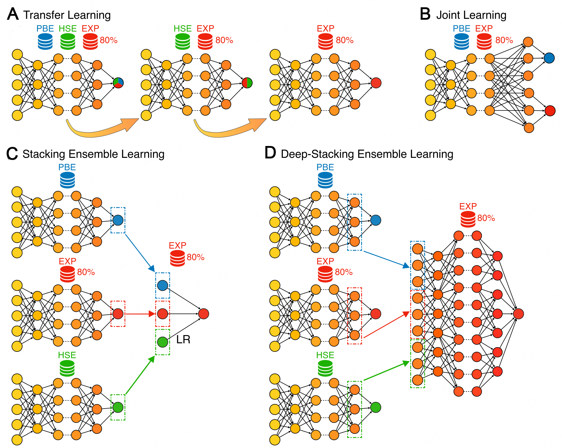
Figure 2. Schematic of the different multi-fidelity methods. (A) Transfer Learning, a model is sequentially trained on
Here, a MODNet model was first trained on the dataset formed by PBE
Joint Learning: This technique, which is schematically illustrated in Figure 2b, consists of having a single model that predicts multiple targets at once with a shared architecture. It is similar to Transfer Learning, but the properties are learned in parallel rather than sequentially.
This approach can improve the accuracy of the predictions, compared to training a model for each target separately. In our case, instead of training only the EXP dataset, we also used the corresponding PBE values. Although technically nothing prevents it, we chose not to use the corresponding HSE values. Indeed, this would have considerably reduced the size of the training set since Joint Learning requires only the data that are common to all considered datasets to be used (only 325 samples, if considering PBE
Stacking Ensemble Learning: This technique, which is schematically illustrated in Figure 2c, consists of combining the predictions of different (weak) learners (i.e., sub-models). In this work, we trained three submodels, respectively, on the PBE, HSE, and EXP datasets. The predictions of these models are referred to as
Deep-Stacking Ensemble Learning: This technique, which is schematically illustrated in Figure 2d, is based on the previous one. Basically, the last hidden layers of the three neural networks were concatenated and used as the input of a new neural network for the final prediction. This can be seen as a feature extraction procedure, where the last hidden layers are high-level descriptors for the electronic band gap. Therefore, one could, in principle, use another model (e.g., random forest) on top of these extracted features. It has the advantage of having more input information than the stacking ensemble.
PBE as a feature: This technique consists of using the PBE results as an additional feature for the model that is trained on the EXP dataset. Note that, for new predictions, a PBE calculation is thus explicitly needed with this technique. In fact, the HSE results could also have been used as an additional feature. This would, however, reduce the size of the training set since all the structures in the EXP dataset are not necessarily in the HSE one.
Correction Learning: This technique consists of learning the correction that needs to be applied to low-fidelity data to obtain a high-fidelity one. Here, we thus used the difference
RESULTS
Band gap results using the multi-fidelity models
As shown in Table 1, MODNet performed particularly well on experimental datasets, which is what materials scientists are looking for. In this section, we focus on how we can further improve predictions of the experimental band gap using knowledge from DFT predictions.
Table 2 summarizes the MAE scores of band gaps using the different multi-fidelity methods. The MODNet model trained only on the EXP dataset shows a MAE of 0.382 eV (note that the dataset is different from the one in Table 1). It is chosen as the reference baseline against which all multi-fidelity learning techniques are compared.
MAE on the band gap for the different multi-fidelity learning techniques (see Figure 2) and for various training and test sets (
| Learning technique | Training sets | Samples | Test set (5-fold) | MAE | |
| Single-Fidelity | EXP | 2480 | EXP | 0.382 | 0% |
| Single-Fidelity | EXP | 4604 | EXP | 0.366 | -4% |
| Transfer Learning | PBE | 2480 | EXP | 0.397 | +4% |
| Joint learning | PBE | 2480 | EXP | 0.368 | -4% |
| Stacking Ensemble Learning | PBE | 2480 | EXP | 0.367 | -4% |
| Deep-Stacking Ensemble Learning | PBE | 2480 | EXP | 0.370 | -3% |
| PBE as a feature | PBE | 2480 | EXP | 0.371 | -3% |
| Correction Learning (PBE) | PBE | 2480 | EXP | 0.318 | -17% |
| Single-Fidelity | PBE | 325 | HSE | 0.582 | 0% |
| Correction Learning (PBE) | PBE | 325 | HSE | 0.442 | -24% |
| Correction Learning (HSE) | PBE | 325 | HSE | 0.402 | -31% |
| Single-Fidelity | EXP | 4604 | HSE | 0.438 | 0% |
| Correction Learning (PBE) | PBE | 2480 | HSE | 0.356 | -19% |
| Correction Learning (HSE) | HSE | 325 | HSE | 0.402 | -8% |
Despite the fact that it only contains the compositions, the MODNet model trained on the more-populated EXP
Most of the investigated learning techniques do not overcome this threshold. Transfer Learning even leads to a deterioration by 4%. The other techniques lead to an improvement of 3–4%, similar to what can be obtained by exploiting all the data with the compositions. On the contrary, the Correction Learning technique based on PBE calculations induces a strong enhancement of 17
Based on these findings, we further investigated whether Correction Learning based on HSE calculations, which are known to provide more accurate estimates of the experimental band gaps, improves the results further or not. To this end, we performed two series of tests. In the first, the training set was purposely limited to HSE
In the first case, the Correction Learning technique led to an improvement of 24
However, in a real situation, such higher-fidelity data (here, the HSE band gaps) are scarcer than lower-fidelity ones. Therefore, we further benchmarked the method taking into account all available data. Three realistic scenarios were considered: (ⅰ) a composition MODNet model trained on the full experimental dataset (4604 compositions); (ⅱ) Correction Learning based on PBE calculations (2480 structures); and (ⅲ) Correction Learning based on HSE calculations (325 structures). Importantly, the three models were tested on a commonly compatible test set: a five-fold test on the inner 325 materials. In this second case, the Correction Learning technique led to an improvement of 19
Finally, it is interesting to note that the same most relevant features are shared among all models (regardless of the target fidelity or strategy such as difference learning). This can be expected as they all are an approximation of the same physical property. They include the element and energy associated with the highest and lowest occupied molecular orbital (computed from the atomic orbitals) and various elemental statistics (such as atomic weight, column number, and electronegativity). The oxidation state also plays an important role in the prediction. The 20 most relevant features are all composition based, with the sole exception of the spacegroup number.
CONCLUSION
In this work, we briefly present an extension of the MODNet model consisting of a new procedure for hyperparameter optimization by means of a genetic algorithm. This approach was shown to be more effective and computationally less expensive. Thanks to this, MODNet outperforms current leaders on 8 out of the 13 Matbench tasks, making it a leading model in material properties predictions.
Furthermore, various techniques relying on multi-fidelity data are presented to improve band gap predictions. These techniques aim to take advantage of all the available data, from limited experimental datasets to large computational ones. Among the various methods investigated, the most promising results were obtained with the Correction Learning technique, which consists of training a model on the difference between the DFT calculations and the experimental measurements. This difference is considered to be a correction to the DFT results. Hence, any new prediction is obtained as the sum of the DFT band gap and the correction predicted by the ML model. Hence, a DFT calculation is still needed, but if PBE is used, it is computationally not very expensive. Among the different models, we studied the trade-off between the accuracy and availability of the computational data. It was concluded that the difference method trained on the PBE dataset yields better performance than the same method applied to scarce but more precise HSE data. In particular, a 17% MAE reduction (with respect to the experimental band gap) was found.
Multi-fidelity correction learning can be applied to various other materials properties, with hopefully similar improvements as obtained here. We therefore encourage and expect that it will be used in a wider context.
DECLARATIONS
Acknowledgments
The authors acknowledge UCLouvain and the F.R.S.-FNRS for financial support. Computational resources have been provided by the supercomputing facilities of the Université catholique de Louvain (CISM/UCLouvain) and the Consortium des Équipements de Calcul Intensif en Fédération Wallonie Bruxelles (CÉCI) funded by the Fond de la Recherche Scientique de Belgique (FRS-FNRS) under convention 2.5020.11 and by the Walloon Region.
Author's contribution
Prepared the different multi-fidelity approaches: De Breuck PP
Implemented and ran the different models: Heymans G
Conceptualized and supervised the work: Rignanese GM
De Breuck PP and Heymans G contributed equally to this work.
All authors contributed to the analysis of the results and the writing of the manuscript.
Availability of data and materials
All the Matbench datasets are available at https://matbench.materialsproject.org. The PBE dataset for the electronic band gap is actually one of those. It can be downloaded from the following URL: https://ml.materialsproject.org/projects/matbench_mp_gap.json.gz. The three other datasets for the electronic band gap are provided as csv files in the Supplementary Material. The MODNet model is available on the following GitHub repository: ppdebreuck/modnet[30].
Financial support and sponsorship
Not applicable.
Conflicts of interest
All authors declared that there are no conflicts of interest.
Ethical approval and consent to participate
Not applicable.
Consent for publication
Not applicable.
Copyright
© The Author(s) 2022.
REFERENCES
1. Magee CL. Towards Quantification of the Role of Materials Innovation in Overall Technological Development. Complexity 2012;18:10-25.
2. Lejaeghere K, et al. Reproducibility in density functional theory calculations of solids. Science 2016;351:aad3000.
3. Himanen L, Geurts A, Foster AS, Rinke P. Data-driven materials science: status, challenges, and perspectives. Adv Sci 2019;6:1900808.
4. Alberi K, Nardelli MB, Zakutayev A, Mitas L, Curtarolo S, et al. The 2019 materials by design roadmap. J Phys D 2019;52:013001.
5. Butler KT, Davies DW, Cartwright H, Isayev O, Walsh A. Machine learning for molecular and materials science. Nature 2018;559:547-55.
6. Schmidt J, Marques MRG, Botti S, Marques MAL. Recent advances and applications of machine learning in solid-state materials science. npj Comput Mater 2019;5:83.
7. Choudhary K, DeCost B, Chen C, Jain A, Tavazza F, et al. Recent advances and applications of deep learning methods in materials science. npj Comput Mater 2022;8:59.
8. Jain A, Ong SP, Hautier G, Chen W, Richards WD, et al. The Materials Project: A Materials Genome Approach to Accelerating Materials Innovation. APL Mater 2013;1:011002.
9. Perdew JP, Burke K, Ernzerhof M. Generalized Gradient Approximation Made Simple. Phys Rev Lett 1996;77:3865-68.
10. Zhuo Y, Mansouri Tehrani A, Brgoch J. Predicting the Band Gaps of Inorganic Solids by Machine Learning. J Phys Chem Lett 2018;9:1668-73.
11. Morales-García Á, Valero R, Illas F. An Empirical, yet Practical Way To Predict the Band Gap in Solids by Using Density Functional Band Structure Calculations. J Phys Chem C 2017;121:18862-66.
12. van Setten MJ, Giantomassi M, Gonze X, Rignanese GM, Hautier G. Automation Methodologies and Large-Scale Validation for G W : Towards High-Throughput G W Calculations. Phys Rev B 2017;96:155207.
13. Heyd J, Scuseria GE, Ernzerhof M. Hybrid Functionals Based on a Screened Coulomb Potential. J Chem Phys 2003;118:8207-15.
14. Kauwe SK, Welker T, Sparks TD. Extracting Knowledge from DFT: Experimental Band Gap Predictions Through Ensemble Learning. Integr Mater Manuf Innov 2020;9:213-20.
15. Chen C, Zuo Y, Ye W, Li X, Ong SP. Learning Properties of Ordered and Disordered Materials from Multi-Fidelity Data. Nat Comput Sci 2021;1:46-53.
16. De Breuck PP, Hautier G, Rignanese GM. Materials property prediction for limited datasets enabled by feature selection and joint learning with MODNet. npj Comput Mater 2021;7:83.
17. Chen C, Ong SP. AtomSets as a Hierarchical Transfer Learning Framework for Small and Large Materials Datasets. npj Comput Mater 2022;7:173.
18. Chen C, Ye W, Zuo Y, Zheng C, Ong SP. Graph Networks as a Universal Machine Learning Framework for Molecules and Crystals. Chem Mater 2019;31:3564-72.
19. Cubuk ED, Sendek AD, Reed EJ. Screening Billions of Candidates for Solid Lithium-Ion Conductors: A Transfer Learning Approach for Small Data. J Chem Phys 2019;150:214701.
20. Goetz A, Durmaz AR, Müller M, Thomas A, Britz D, et al. Addressing Materials' Microstructure Diversity Using Transfer Learning. npj Comput Mater 2022;8:27.
21. Gupta V, Choudhary K, Tavazza F, Campbell C, Liao Wk, et al. Cross-Property Deep Transfer Learning Framework for Enhanced Predictive Analytics on Small Materials Data. Nat Commun 2021;12:6595.
22. Ju S, Yoshida R, Liu C, Wu S, Hongo K, et al. Exploring Diamondlike Lattice Thermal Conductivity Crystals via Feature-Based Transfer Learning. Phys Rev Mater 2021;5:053801.
23. Kong S, Guevarra D, Gomes CP, Gregoire JM. Materials Representation and Transfer Learning for Multi-Property Prediction. Appl Phys Rev 2021;8:021409.
25. Dunn A, Wang Q, Ganose A, Dopp D, Jain A. Benchmarking Materials Property Prediction Methods: The Matbench Test Set and Automatminer Reference Algorithm. npj Comput Mater 2020;6:1-10.
26. Fronzi M, Isayev O, Winkler DA, Shapter JG, Ellis AV, et al. Active Learning in Bayesian Neural Networks for Bandgap Predictions of Novel Van Der Waals Heterostructures. Adv Intell Syst 2021;3:2100080.
27. Pilania G, Mannodi-Kanakkithodi A, Uberuaga BP, Ramprasad R, Gubernatis JE, et al. Machine Learning Bandgaps of Double Perovskites. Sci Rep 2016;6:19375.
28. Rajan AC, Mishra A, Satsangi S, Vaish R, Mizuseki H, et al. Machine-Learning-Assisted Accurate Band Gap Predictions of Functionalized MXene. Chem Mater 2018;30:4031-38.
29. Ward L, Agrawal A, Choudhary A, Wolverton C. A General-Purpose Machine Learning Framework for Predicting Properties of Inorganic Materials. npj Comput Mater 2016;2:16028.
30. MODNet v0.1.9;. https://github.com/ppdebreuck/modnet.
31. De Breuck PP, Evans ML, Rignanese GM. Robust Model Benchmarking and Bias-Imbalance in Data-Driven Materials Science: A Case Study on MODNet. J Phys: Condens Matter 2021;33:404002.
32. Choudhary K, DeCost B. Atomistic Line Graph Neural Network for improved materials property predictions. npj Comput Mater 2021;7:185.
33. Wang AYT, Kauwe SK, Murdock RJ, Sparks TD. Compositionally restricted attention-based network for materials property predictions. npj Comput Mater 2021;7:77.
34. Xie T, Grossman JC. Crystal graph convolutional neural networks for an accurate and interpretable prediction of material properties. Phys Rev Lett 2018;120:145301.
35. Ward L, Dunn A, Faghaninia A, Zimmermann NER, Bajaj S, et al. Matminer: An Open Source Toolkit for Materials Data Mining. Comput Mater Sci 2018;152:60-69.
36. Kingsbury R, Gupta AS, Bartel CJ, Munro JM, Dwaraknath S, et al. Performance comparison of r2SCAN and SCAN metaGGA density functionals for solid materials via an automated, high-throughput computational workflow. Phys Rev Mater 2022;6:013801.
Cite This Article

How to Cite
Download Citation
Export Citation File:
Type of Import
Tips on Downloading Citation
Citation Manager File Format
Type of Import
Direct Import: When the Direct Import option is selected (the default state), a dialogue box will give you the option to Save or Open the downloaded citation data. Choosing Open will either launch your citation manager or give you a choice of applications with which to use the metadata. The Save option saves the file locally for later use.
Indirect Import: When the Indirect Import option is selected, the metadata is displayed and may be copied and pasted as needed.
About This Article
Copyright


Comments
Comments must be written in English. Spam, offensive content, impersonation, and private information will not be permitted. If any comment is reported and identified as inappropriate content by OAE staff, the comment will be removed without notice. If you have any queries or need any help, please contact us at support@oaepublish.com.