


Revised dynamic climate change impact assessment for life cycle assessment through delay factors expressions
 0
0 
Abstract
Dynamic Life Cycle Assessment (LCA) ranges in temporal complexity, with fully dynamic approach requiring full life-cycle chronologies for both foreground and background systems. For instance, LCAs based on Environmental Product Declaration (EPDs), required by the French RE2020 regulation, are partially dynamic, since only the foreground timeline is available. The goal of this research is to provide a user-friendly and rigorous method to conduct partially dynamic LCAs for climate change impact based on EPDs. Delay factors are built as coefficient depending on the time distribution of emissions, to define the dynamic characterization factor as a function of the static one. Compatibility constraints between static and dynamic imposes an observation time T equal to the sum of the Life Cycle Duration (LCD) and the Time Horizon of the Impact (THI). Literal mathematical expressions of delay factors and their behaviors are provided for Global Warming Potential (GWP) and Global Temperature Potential (GTP). The application scope of these delay factors covers all greenhouse gases (GHG) and large temporal range of LCD and THI. A case study based on three background products and randomly generated foreground emissions shows that the RE2020 regulation dynamic factors overestimate benefits obtained by delaying emissions compared to present method. This happens because the method ignores compatibility constraints between static and dynamic approaches and because it does not differentiate delay factors for distinct GHGs. However, delaying emissions reduces GWP but still raises GTP, questioning the use of GWP as a dynamic indicator, as it may falsely suggest a declining impact when it is actually increasing.
Keywords
INTRODUCTION
Dynamic Life Cycle Assessment (LCA) covers the notion of taking temporality explicitly into account in an LCA study. More precisely, a dynamic LCA is defined as the combination of two models: (i) a dynamic life cycle inventory (LCI), modelling time-dependent processes in the technosphere; and (ii) a dynamic life cycle impact assessment (LCIA), representing the time-varying nature of the expected effects within the ecosphere[1]. Dynamic LCA is not specific to climate change, but it has been initially developed concerning that specific impact category[2,3]. Each impact category would require a very different dynamic characterization approach, depending on the underlying impacted natural phenomena. However, only few studies jointly implement both a dynamic inventory and a dynamic climate-change characterization, despite the methodological need for doing so[4].
LCA approaches regarding climate change assessments have been classified into four categories for time accounting[5]: (1) Purely static approaches, with no consideration for time; (2) Partially dynamic approaches combining a static inventory and an LCIA with credit for carbon storage; (3) Partially dynamic approaches, where a dynamic inventory is assessed through a static LCIA method, and (4) Fully dynamic approaches based on both a dynamic LCI and LCIA. For the sake of clarity, instead of using these categories as defined by[5], we prefer to refer in the remainder of this article to static, partially dynamic and fully dynamic approaches, as illustrated in Figure 1. A partially dynamic approach is characterized by a temporally explicit foreground LCI, whereas a fully dynamic approach involves a temporally explicit inventory for both the foreground and background LCIs. In either case, the LCIA is temporally explicit.
Figure 1. Illustration of levels of difficulties of time explicit LCAs from static to dynamic - *categories as defined by[5] - ** “delay factor” is an expression used and precisely defined later in the present article, the current expression employed by[5] “discount factor”. LCAs: Life cycle assessment.
For a fully dynamic approach, a basic understanding of the chronological progression of life cycle processes in the foreground system and/or the temporal equations is insufficient. It is also essential to be able to temporally align all background system processes with respect to those in the foreground system, i.e. “to combine the different dynamics of the unit processes together”[6]. An example of this issue is provided in Figure 1 for the case of a building. It is required to trace back in time the production of each composing material, and then further in time their use and end-of-life flows relative to the construction timeline. Similarly, each intermediate flow required by the production processes of these composing materials has to be traced in time relatively to the production, use and end-of-life times of this specific material, etc. Such an approach requires a mathematical framework and a computing method able to recreate a chronological database from the temporal description of a product life cycle. Additionally, temporal LCI models can vary in complexity, ranging from basic chronological ordering of processes to more complex dynamic relationships. In the latter case, the value of an inventory flow at a given time t is a function of its value at the preceding time step, as exemplified by models of biomass growth in silviculture. Two types of approaches, grounded in distinct mathematical techniques, have been put forward to address this issue: the first relies on the method of limited expansion[7], while the second utilizes dynamic graph search algorithm[6]. These have later been improved and operationalized[8-10]. However, these fully dynamic methods can only be implemented on specific databases for which all the intermediate flows are available (such as unit process models in the ecoinvent database). Their implementation also demands a high level of programming expertise.
Recently, some new regulations, such as the RE2020 in France[11], impose to stakeholders of the building sector the calculation of a dynamic indicator based on Environmental Product Declaration (EPDs). However, for operational approaches based on EPDs, only partially dynamic approaches are possible. Indeed, as illustrated in Figure 1, LCAs of products from EPDs are aggregated without the detail of the background processes models that is needed to recreate a fully time-explicit LCI. Thus, only the foreground system is time explicit, whereas the background (i.e. any upstream intermediate and elementary flows) will be considered as being produced at the same time as the EPD product. Referring to the illustration in Figure 1, there is no possibility of moving from a partially dynamic to a fully dynamic approach with EPDs. Performing dynamic LCA using EPDs is thus based on a major simplifying assumption: the “temporal alignment” of EPDs’ inventories, i.e. considering that the LCA of an EPD product takes place entirely at the very same time. This implies that the background system is static while the foreground system is dynamic. This “bonding” between a static background system and a dynamic foreground system requires the ability to calculate a dynamic indicator from a static indicator, and that both static and dynamic indicators to be mathematically compatible.
Previous work has been published to ease the implementation of partially dynamic LCAs applied to climate change impact category. A worksheet-based tool[12] based on the work of Levasseur et al. is very operational for practitioners but provides characterization factors based on the 5th IPCC report (Intergovernmental Panel on Climate Change)[13]. In addition, the tool is not transparent enough to be adaptable to further evolutions from IPCC because the calculation model of delay and characterization factors is not fully provided. Furthermore, because it is based on a numerical model, the results are dependent on the chosen time-step, that influences both results and computation time[14]. More recently, Resch et al. provided an operational relationship between Global Warming Potential (GWP) static and dynamic indicators, but this remains an empirical approximation[15]. In both approaches, the integration times of radiative effects associated with the inventory and with the reference gas are indeed critical components of the dynamic GWP metric. They strongly influence climate-change outcomes, particularly for short-lived pollutants such as CH4 and N2O, and may result in the truncation of radiative effects for emissions occurring later in the life cycle[16,17]. However, both approaches only consider the GWP indicator, although Global Temperature Potential (GTP) gains interest in today’s scientific and political discussions, and is subject to the same time-horizon limitations as GWP[18,19]. Additionally, neither approach guarantees the existence of a mathematical consistency between the static indicators of the background system and the dynamic indicators of the foreground system. Other existing climate indicators do not rely on fixed time horizons or a reference gas - such as the integrated global mean temperature change (iGMTC), the amplitude of the temperature change (GMTCmax), the ΔTpeak or the ΔTlong-term - and therefore provide unbiased metrics of climate change, but their applications require a fully dynamic inventory[20,21].
The goal of this research is to provide a user-friendly method enabling practitioners to conduct partially dynamic LCAs for climate change impact based on EPDs, making it accessible to a wider range of stakeholders. Beyond operational simplicity, the contribution of this work also lies in establishing analytical coefficients that can be applied directly to static characterization factors to obtain their dynamic counterparts. Because these coefficients depend on a consistent alignment of time horizons between static and dynamic formulations, the method explicitly derives and formalizes the required compatibility conditions. Although developed primarily for GWP - the only climate change indicator currently reported in EPDs - the approach is extended to GTP to anticipate potential shifts in climate policy and impact assessment practice.
The remainder of this article is structured as follows. Section 2 introduces the climate change modelling principles underlying GWP and GTP indicators, including the definition of main time horizons. Section 3 derives mathematical expressions of so-called “delay factors” - coefficients that depend on the temporal distribution of emissions and that scale the static characterization factor to obtain the dynamic one for the same system. In parallel, their behaviors as a function of their input parameters are analyzed. Section 4 presents a simple application of the method, together with its associated worksheet-based tool[22], using EPD data within the framework of the French RE2020 regulation. Section 5 discusses the physical meaning of delay factors along with their operability and reliability.
PRINCIPLES OF CLIMATE CHANGE INDICATOR AND MAIN DYNAMIC METHODS
This section presents the principles and main equations, introducing unified notations and symbols. To avoid repetition and verbosity in the text, all notations and their units are detailed in the Supplementary Table 1.
General principles of climate change metrics modeling
Assessing and modelling the potential impacts of greenhouse gases (GHG) emissions on climate change rely on a complex methodological process starting with the inventory of atmospheric GHG emissions. Higher atmospheric concentrations of GHGs lead to stronger radiative forcing. Changes in energy intake changes atmospheric temperature which in return affects climate conditions such as terrestrial and ocean temperatures, or the sea level. Finally, these new climate conditions create potential damages on human health, ecosystem quality or natural resources[23]. Throughout this cause-effect chain, many indicators can be suggested to represent climate change: from emissions accounting to damage indicators, including radiative forcing, temperature, sea level or even precipitation metrics. The indicators used can be differentiated according to their absolute or relative nature, or according to their underlying temporal approach - instantaneous or cumulative.
The following equations are those provided by the IPCC. For the reader's convenience, the meaning and units are fully detailed in the Supplementary Table 1.
Both GWP and GTP indicators are based on the Absolute Global Forcing Potential (AGFP). It represents the amount of radiative power received by 1 m2 of Earth surface due to a pulse increase of 1 kg of a given GHG. The AGFP is an instantaneous metric of the radiative forcing:
with AGFPj(t) the Absolute Global Forcing Potential (W.m-2.kg-1); cj the time response function of an impulse of the GHG j (dimensionless), aj is the radiative efficiency of GHG j (W.m-2.kg-1) and t the time elapsed after the pulse emission[24].
The time decay law, or impulse response function, cj(t) represents the degradation of the GHG j over the time (or its reabsorption by biogeochemical mechanisms regarding the CO2):
with cj the time response function of an impulse of the GHG j (dimensionless), τj the lifetime of the GHG j in the atmosphere (years) and bn and τn the carbon dioxide impulse response function parameters taken from[25].
Lifetimes of all GHGs are provided in an associated worksheet-based tool[22], under the “IPCC AR6” worksheet based on[26,27], bn and τn are provided in the “Additional data” worksheet based on[25].
The Absolute Global Warming Potential (AGWP) is the instantaneous radiative forcing [Equation 2] cumulated over a time T:
with AGWPj(T) the Absolute Global Warming Potential of GHG j cumulated over a time T (W.m-2.yr.kg-1)[24].
The GWP characterization factor is a relative metric based on the AGWP expressed relatively to the CO2 chosen as the reference substance:
with GWPj(T) the static Global Warming Potential characterization factor of GHG j over time T
The Absolute Global Temperature Potential (AGTP) represents the temperature variation due to the radiative forcing potential, expressed in Equation 5[24]. It is based on the AGFP and on a temperature response function. Compared to the radiative forcing, a temperature variation is introduced that relies on the climate impulse response Rθ. This one is based on climatic layers models. In latest IPCC reports, AR5 and AR6, Rθ is represented by a two exponential terms expression with a fast and a slow contribution, as expressed in Equation 6[28].
with AGTPj(T) the Absolute Global Temperature Potential of GHG j over a time T (K.kg-1) and Rθ(t) the climate warming impulse response function (K.yr-1.m2.W-1)[24].
The climate warming impulse response function Rθ is expressed as follows:
with qs, qf, (K.m2.W-1) representing respectively a slow and a fast contribution to the temperature increase in respectively ds and df (year) the surface and deep layers of the atmosphere[28].
The GTP indicator, in Equation 7, is a relative metric based on the AGTP expressed relatively to the CO2, chosen as a reference substance.
with GTPj(T) the Global Temperature Potential indicator of GHG j over a time T (kg CO2-eq)[24].
In addition to the degradation or absorption rates of GHGs and their climate impulse responses, some feedback mechanisms contribute to climate change metrics. Firstly, through oxidation reactions, a part of methane emissions degrades into carbon dioxide. These indirect emissions contribute to climate change and are estimated through the cumulative product of methane degradation and AGWP of CO2 (see Equations in Supplementary Part 2). Secondly, any GHG emissions that contribute to global warming can modify the balance of carbon flows between Earth’s reservoirs. Then for each GHG other than CO2, metrics should integrate a carbon cycle response.
Dynamic metrics for climate change
To distinguish dynamic factors from static ones, static quantities are indicated in upper case in the previous section, and dynamic quantities in lower case in the following section.
Unified mathematical framework between static and dynamic approaches
In this section, several time entities are defined. The times corresponding to the first and last emission of the life cycle of the considered product are defined as t0 and tmax respectively. Then, the duration of the LCD (life cycle duration) can be defined as:
with LCD the Life Cycle Duration (yrs), t0 (yrs) the time of the first emission of the life cycle, and tmax(yrs) the last emission of the life cycle.
Let’s also define tx as the time at which the integration calculation stops. Thus, independently from the static or dynamic method, the total integration time can be expressed as:
For static impact assessment, as represented in Figure 2A, the integration time is equal to the Time Horizon of the Impact:
Figure 2. Comparison of static and dynamic approaches. GHG: Greenhouse gases; LCD: life cycle duration.
Figure 2B shows the same case study with a dynamic approach: all emissions of the inventory system model are now spread between t0 and tmax. The total integration time corresponding to Equation 9 can be rewritten by introducing tmax as follows:
To build a unified framework between static and dynamic approaches, the static equation should be derived from the dynamic one. By setting tmax = t0, corresponding to all emissions occurring at time t0, expressions of T are equals:
Giving therefore the following relationship for the static expression:
Which finally leads to the unified expression:
This condition is general to any impact category whenever compatibility is required between static and dynamic approaches. This relationship had already been suggested and conceptually explained by[29] although it was not demonstrated. For partially dynamic approaches based on EPDs, Time Horizon of the Impact (THI) = 100 years.
Dynamic GWP characterization factors
On a general basis, the agwp of a GHG j emitted at time ti over an observation duration T can be deduced from Equation 3 by introducing the time ti at which the emission occurs:
where agwpi,j(T) is the dynamic Absolute Global Warming Potential of GHG j emitted at time ti and cumulated over time T (W.m-2.yr-1.kg-1).
To obtain dynamic gwp characterization factor, one requires to divide dynamic agwp by the agwp of 1 kg of the reference substance (carbon dioxide). Thus, considering the equivalence of notation between
where gwpi,j(T) is the dynamic Global Warming Potential of GHG j emitted at time ti and cumulated over time T (kg CO2-eq).
Dynamic GTP characterization factors
Like GWP, the dynamic agtp and gtp characterization factors can be expressed from the static AGTP and GTP, Equations 5 and 7 respectively, by introducing the time of emission ti as expressed in Equations 17 and 18:
where agtpi,j(T) is the dynamic Absolute Global Temperature Potential of GHG j emitted at time ti and cumulated over time T (K.kg-1).
where gtpi,j(T) is the dynamic Global Temperature Potential of GHG j emitted at time ti and cumulated over time T (kg CO2-eq).
DELAY FACTORS
Definition
In order to compare and easily convert characterization factors from static to dynamic, the delay factors, symbolized by α and β respectively for the gwp and gtp are defined as dimensionless coefficients representing the ratio between the dynamic and the static characterization factors, for each type of GHG, at a given moment of emission ti and for a given integration time T. Given that CO2, CH4 and N2O represent the overwhelming share of climate‑forcing emissions globally, the differing behaviors of α and β are particularly relevant for these three gases. This is demonstrated in the case study in Section 4 and documented in Supplementary Part 3 and Supplementary Figures 1-4.
Delay factor α for the global warming potential characterization factor
By definition, the delay factor α is expressed as:
Replacing in Equation 19 the corresponding expressions for the GWP and gwp respectively from Equations 4 and 16, while considering the equivalence of notation agwpo,j(T) = AGWPj(T), the following simplified expression is obtained:
Moreover, combining Equation 2 that represents the degradation rates of GHGs, and Equation 20, and resolving the integral, leads to Equation 21 below. The detailed mathematical demonstration is available in Supplementary Part 3.1.
Equation 21 shows that, for other gases than CO2, the delay factor αi,j(T) depends on only one specific gas constant that is τj corresponding to the lifetime of the GHG j, which represents its persistence in the atmosphere. It does not depend on the radiative efficiency nor the molecular mass of the GHG. It does not depend either on any constants relative to CO2 although this is the reference substance of the GWP indicator.
Figure 3 and Table 1 illustrate the variability of αi,j(T) according to the lifetime of a given GHG j, assuming its emission at the end of the Life Cycle Duration, e.g. ti = LCD, and for a Time Horizon of Impact set to THI = 100 years. Eleven current GHGs are plotted on this figure. Figure 3 shows that the higher the lifetime, the smaller the delay factor. This means that delaying emissions of long-lifetime GHGs is more efficient to reduce the indicator.

Figure 3. Delay factors for GWP as a function of the lifetimes of GHGs and for a single emission ti = LCD with THI = 100 years. GHG: Greenhouse gases; LCD: life cycle duration; THI: time horizon of the impact; GWP: global warming potential.
Delay factors for GWP for the 11 main GHG and for a single emission ti = LCD with THI = 100 years
| GHG | Lifetime | Alpha factor (LCD = 10 yrs) | Alpha factor (LCD = 25 yrs) | Alpha factor (LCD = 50 yrs) | Alpha factor (LCD = 100 yrs) | Alpha factor (LCD = 200 yrs) |
| CO2 | Combined | 0.928 | 0.84 | 0.728 | 0.581 | 0.432 |
| CH4 with oxidation | 11.8 | 0.994 | 0.986 | 0.972 | 0.948 | 0.907 |
| N2O | 109 | 0.945 | 0.88 | 0.803 | 0.715 | 0.641 |
| HFC-134a | 14 | 1 | 0.999 | 0.999 | 0.999 | 0.999 |
| HFC-125 | 30 | 0.99 | 0.98 | 0.971 | 0.966 | 0.964 |
| SF6 | 1000 | 0.914 | 0.81 | 0.683 | 0.525 | 0.367 |
| PFC-14 | 50000 | 0.909 | 0.8 | 0.667 | 0.5 | 0.334 |
| CFC-11 | 52 | 0.971 | 0.939 | 0.904 | 0.872 | 0.857 |
| CFC-12 | 102 | 0.947 | 0.885 | 0.811 | 0.727 | 0.66 |
| HCFC-22 | 11.9 | 1 | 1 | 1 | 1 | 1 |
| CCl4 | 32 | 0.988 | 0.976 | 0.965 | 0.958 | 0.956 |
Figure 4 depicts the evolution of the delay factor αi,j(T) as a function of the Time Horizon of the Impact THI for a single emission occurring at the time ti = LCD with LCD = 100 years. The three time horizons classically used for the GWP indicator (20,100 and 500 years) are also marked on the figure. One can observe that all delay factors are close to zero for short Time Horizons of the Impact and eventually tend towards 1 at long Time Horizons of the Impact. The shorter the GHG lifetime, the faster they approach 1.
Figure 4. Delay factors for GWP as a function of the Time Horizon of the Impact (THI) and for a single emission ti = LCD=100 years. GHG: Greenhouse gases; LCD: life cycle duration; GWP: global warming potential.
Figure 5 shows different values of the delay factor for CO2 emissions αi,CO2(T) , as a function of the time of emission ti, with a Time Horizon of Impact set to THI = 100 years for four Life Cycle Duration LCD scenarios (25, 50, 100 and 200 years). Similar figures for CH4 and N2O are provided in Supplementary Figures 1 and 2. As the time of emission ti and Life Cycle Duration LCD increase, the delay factor decreases, which means that for a given Time Horizon of the Impact, later emissions have a lower impact GWP indicator. Nonetheless, increasing the LCD period decrease the slope of delay factors, then delayed emissions occurring before LCD will have less favorable delay factors than with a shorter LCD.

Figure 5. Delay factors for GWP of CO2 as a function of the time of emission for a Time Horizon of the Impact (THI = 100 years) and for various Life Cycle Durations (LCD). GWP: Global warming potential
Delay factor β for global temperature potential characterization factor
As defined before, the mathematical expression of the delay factor β associated to the GTP indicators for a given observation time T is:
Similarly to the delay factor α [Equation 20], Equation 22 can be rewritten by replacing the expression of Equations 5 and 18, while considering the relationship agtp0,j(T) = AGTPj(T):
As with the GWP, from combination of Equations 2, 6, 17 and 23, the delay factor for the GTP can be expressed analytically for each GHG j, for each moment of emission ti and any integration time T. The detailed mathematical demonstration is available in Supplementary Part 3.2.
Similar to GWP, Equation 24 shows that for other gases than CO2, the delay factor βi,j(T) exclusively depends on the lifetime of the GHG for gas-specific constants and on the four constants related to the climate impulse response[28]. Nor does it depend on any constants relative to CO2 although this is the reference substance of the GTP indicator.
Figure 6 and Table 2 illustrate the variability of βi,j(T) according to the lifetime of a GHG j, assuming they are emitted at the time ti corresponding to the end of the Life Cycle Duration (ti = LCD ) and for a Time Horizon of Impact set to THI = 100 years. Eleven current GHGs are plotted on this figure. One can observe in Figure 6 that the delay factor increases up to a maximum for GHGs lifetimes between 10 and 50 years, and decreases down to one for lifetimes between 50 and 1,000 years, then below one for lifetimes longer than 1,000. The maximum value of the delay factor increases with the value of the life cycle duration LCD. As displayed on Figure 6 related to THI = 100 years, whatever the value of LCD, the delay factor is superior to 1 for all GHGs with lifetimes of less than 600 to 1,000 years depending on whether LCD varies between 10 and 200 years. This means that, unless the lifetime of the GHG in the atmosphere is greater than 1,000 years, the longer an emission is delayed, the greater the temperature rises 100 years after the last emission.
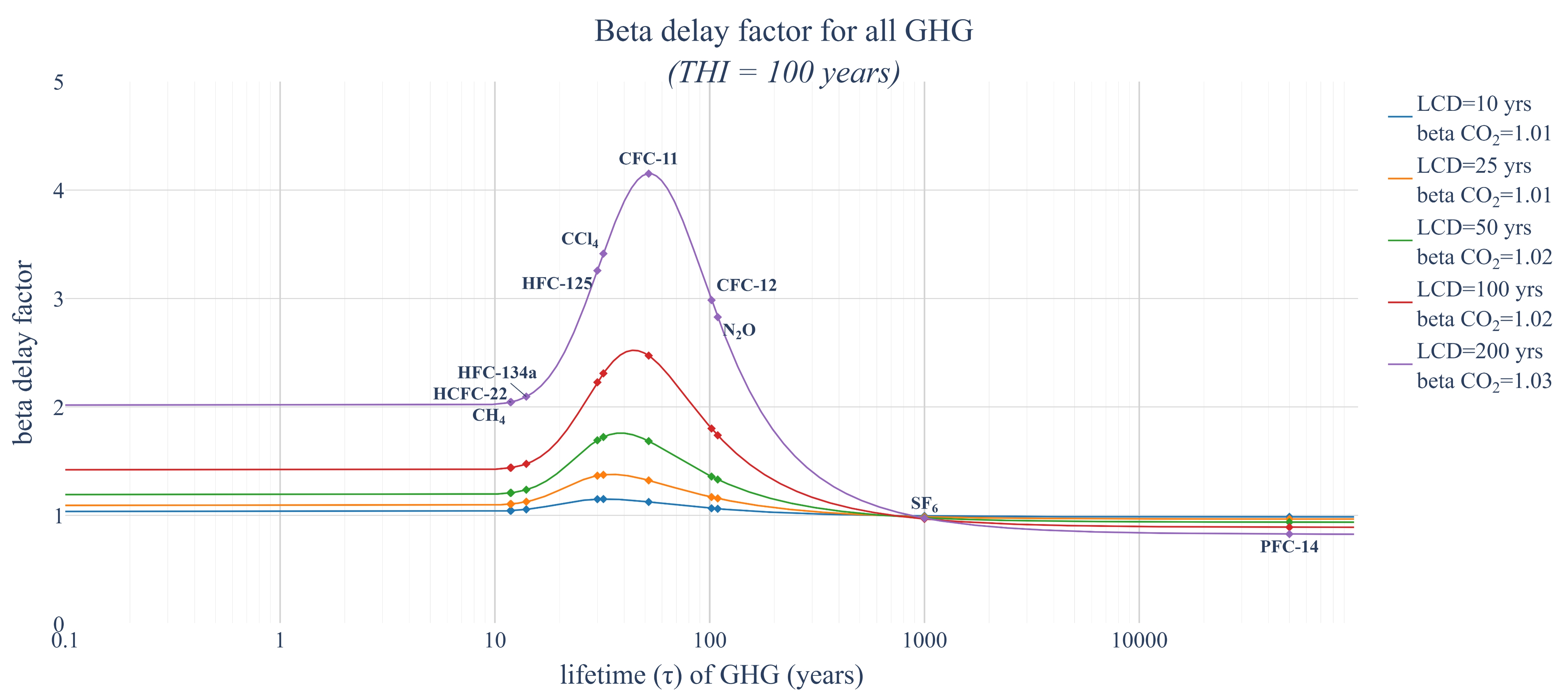
Figure 6. Delay factors for GTP as a function of the lifetimes of GHGs and for a single emission ti = LCD with THI = 100 years. GHG: Greenhouse gases; LCD: life cycle duration; THI: time horizon of the impact; GWP: global warming potential; GTP: global temperature potential.
Delay factors for GTP for the 11 main GHG and for a single emission ti = LCD with THI = 100 years
| GHG | Lifetime | Beta factor (LCD = 10 yrs) | Beta factor (LCD = 25 yrs) | Beta factor (LCD = 50 yrs) | Beta factor (LCD = 100 yrs) | Beta factor (LCD = 200 yrs) |
| CO2 | Combined | 1.006 | 1.011 | 1.016 | 1.02 | 1.032 |
| CH4 with oxidation | 11.8 | 1.034 | 1.08 | 1.155 | 1.312 | 1.672 |
| CH4 | 11.8 | 1.043 | 1.104 | 1.207 | 1.439 | 2.043 |
| N2O | 109 | 1.06 | 1.156 | 1.331 | 1.738 | 2.828 |
| HFC-134a | 14 | 1.55 | 1.126 | 1.236 | 1.475 | 2.095 |
| HFC-125 | 30 | 1.149 | 1.366 | 1.692 | 2.227 | 3.257 |
| SF6 | 1000 | 0.994 | 0.987 | 0.977 | 0.967 | 0.974 |
| PFC-14 | 50000 | 0.986 | 0.966 | 0.937 | 0.891 | 0.828 |
| CFC-11 | 52 | 1.124 | 1.323 | 1.684 | 2.473 | 4.151 |
| CFC-12 | 102 | 1.065 | 1.169 | 1.358 | 1.801 | 2.985 |
| HCFC-22 | 11.9 | 1.044 | 1.105 | 1.208 | 1.44 | 2.045 |
| CCl4 | 32 | 1.15 | 1.374 | 1.722 | 2.309 | 3.413 |
Figure 7 depicts the evolution of the delay factor βi,j(T) as a function of the Time Horizon of the Impact THI for a single emission occurring at the time ti = 100 years (i.e. LCD = 100 years). Two time-horizons (50 and 100 years) are also marked on the figure. One can observe that all delay factors tend towards 1 at long Time Horizons of the Impact. For short Time Horizons of the Impact, only GHGs with very long lifetimes have delay factors of less than 1, while GHGs with short lifetimes have significantly higher delay factors.
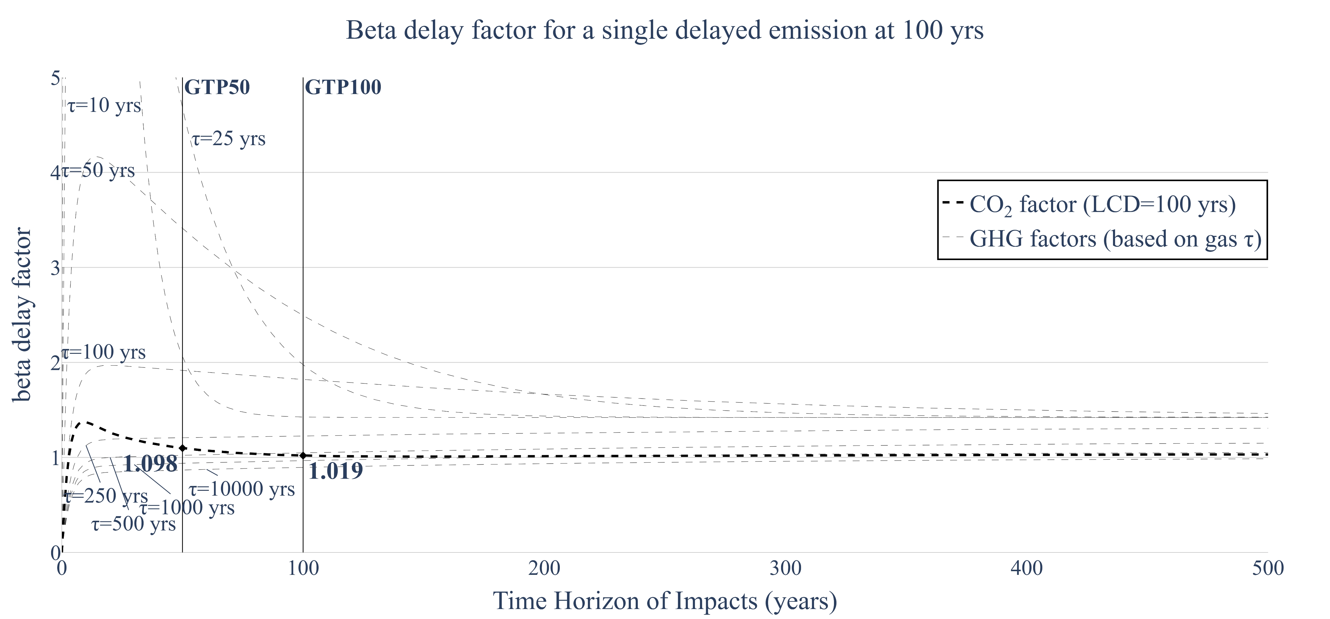
Figure 7. Delay factors for GTP as a function of the Time Horizon of the Impact (THI) and for a single emission ti = LCD = 100 years. GTP: Global temperature potential; LCD: life cycle duration; GHG: greenhouse gases.
Figure 8 shows different values of the delay factor βi,CO2(T) for CO2 emissions, as a function of the emission time ti, with a Time Horizon of Impact set to THI = 100 years, for four LCD scenarios (25, 50, 100 and 200 years). Similar figures for CH4 and N2O are provided in Supplementary Figures 3 and 4. As the time of emission ti and Life Cycle Duration LCD increase, the delay factor increases, which means that for a given THI, later emissions have a higher GTP impact. Additionally, the delay factor is almost constant and very close to 1 for all emission times ti in their variation range (e.g., ti between zero and LCD). This means that delaying CO2 emissions would induce only a slight increase of the GTP indicator, yet for CH4 and N2O the GTP indicator increases significantly with delayed emissions (see Supplementary Figures 3 and 4).
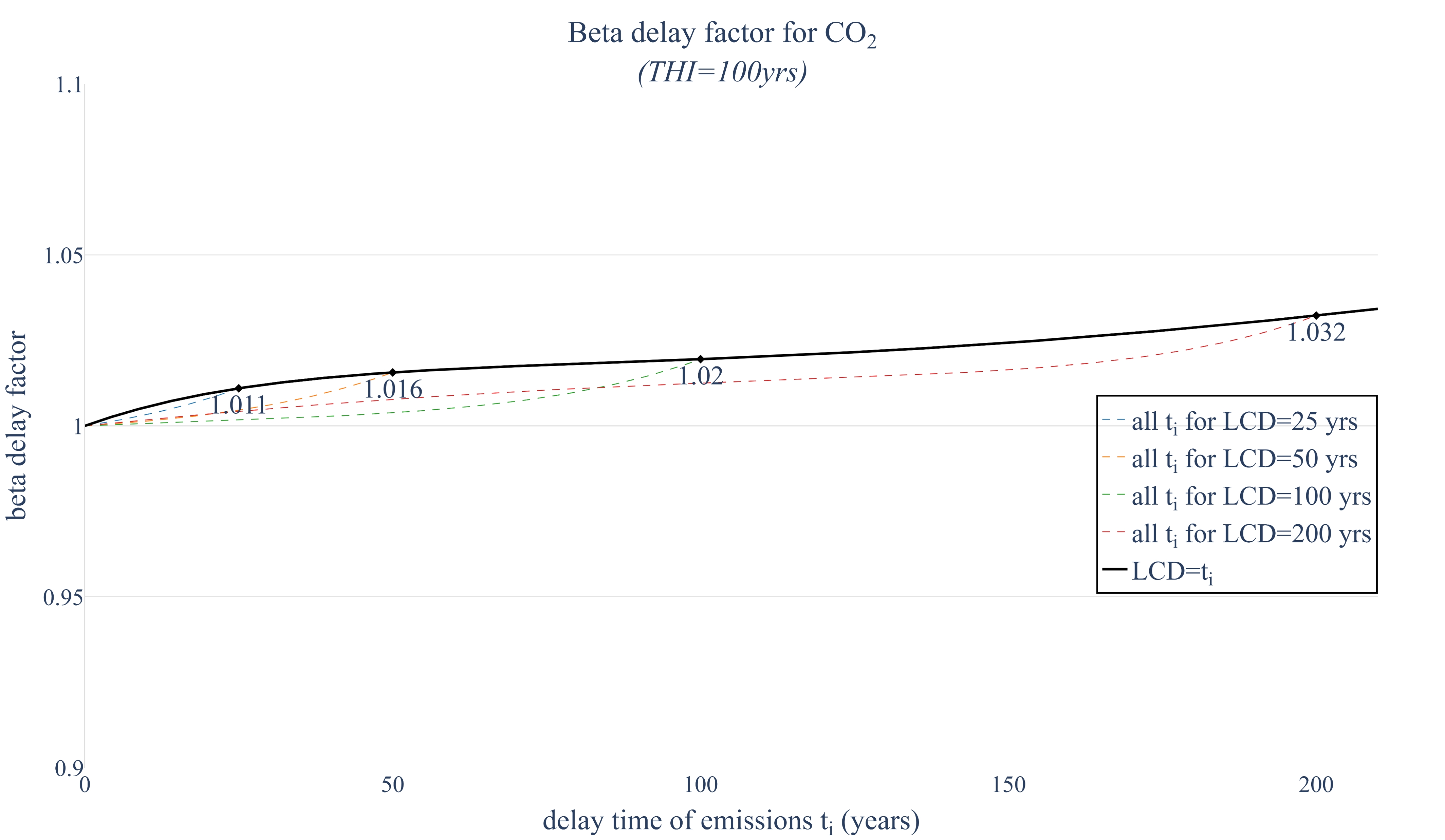
Figure 8. Delay factors for GTP of CO2 as a function of the time of emission ti for a Time Horizon of the Impact (THI = 100 years) and for various Life Cycle Durations (LCD). GTP: Global temperature potential.
Application
This section aims to illustrate how to apply the method and provided tool, for stakeholders who need to conduct a dynamic study using EPDs in compliance with the French RE2020 regulation[11]. This regulation is based on the GWP100 indicator available from EPDs, setting THI = 100 years. This regulation also sets the life of a building at 50 years, setting LCD = 50 years. Year zero is set as the year of delivery of the finished building, and year 50 is set as the year of demolition. Also, according to this regulation[11,30], all operations prior to delivery are set at year zero, and all operations after the year of demolition are set at year 50.
For the purpose of providing an illustrative application of our development, delay factor calculations are thus carried out for three background products (with known EPDs) and one foreground activity, that could be used in a real-life LCA of a building that should comply with the French RE2020 regulation[11]. The delay factors are exact analytical results requiring no empirical validation, and such case study serves to demonstrate the operational workflow and quantify the gap with RE2020. The three background products represent types of products most commonly involved in these regulatory calculations: a material with a long service life used for building construction and not renewed during the building use phase, a material with a short service life used for the building construction and renewed during the building use phase, and a fuel used for heating the building throughout its lifespan. Additionally, a foreground inventory is also randomly generated at every time step to represent a dynamic model supposed to be known and specifically defined by the building designer. Randomly generated foreground emissions were deliberately chosen to demonstrate the generality of the approach, independently of any specific industrial scenario. Then our case study illustrates a partially dynamic study, with temporally defined intermediate flows (background products), and elementary flows (randomly generated).
The regulation RE2020 being based on EPDs data, the life cycle stages of products are named accordingly in the example: module A for production and installation, module B for usage phase, and module C for end-of-life stage[31].
Description of the case study
To avoid citing a specific supplier, default environmental data provided by the French Ministry of Ecological Transition and available in the INIES database are used. A timber frame wall[32] is chosen as a long-life material, a wallpaper for walls and ceilings is chosen as a short-life material, and a wood pellet heating system[32] is chosen for heating energy. Table 3 presents their main characteristics together with their GWP100 values, as well as the associated discrete event time points (i.e., installation, replacement, disposal and energy consumption). Using these data, it is possible to reconstruct a partially dynamic inventory in accordance with the rules set forth by RE2020[11,30] and explained below.
Data used to calculate the partially dynamic GWP indicator in the context of the French regulation RE2020
| Building component | Service life | Reference of EPD | Reference flow | Amounts of products and scenario | Module A | Module B | Module C |
| Timber frame wall | 100 years | (INIES, 2022) | 1 m2 | 50 m2 | |||
| Static GWP | GWP100 (kg CO2 eq) | -7.63 | 0 | 25 | |||
| Timeline scenario | Time 0 | 50 m2 | |||||
| Time 50 | 50 m2 | ||||||
| Wallpaper for walls and ceilings | 10 years | (INIES, 2019) | 1 m2 | 35 m2 | |||
| Static GWP | GWP100 (kg CO2 eq) | 0.970 | 0 | 0.0416 | |||
| Timeline scenario | Time 0 | 35 m2 | |||||
| Every 10 year (Time = 10, 20, 30, 40) | 35 m2 each time | 35 m2 each time | |||||
| Time 50 | 35 m2 | ||||||
| Wood pellet heating system | - | (INIES, 2021) | 1 kWh | 2,500 kWh | |||
| Static GWP | GWP100 (kg CO2 eq) | 0.030 | |||||
| Timeline scenario | Time 0 | 2,500 kWh | |||||
| Every year | 2,500 kWh per year | ||||||
| Time 50 | 2,500 kWh | ||||||
| Foreground specific product | Random data for this example | 1 kg | 1 kg | Specific data detailed by GHG collected by stakeholder | |||
For materials with a long lifespan (greater than or equal to 50 years), the value of module A should be reported at time zero, the value of Module B should be uniformly distributed over the entire lifespan of the building, and the value of Module C should be reported at the end of the building’s life. The impact values are multiplied by the amount of flow necessary for the building. The wall surface is set at 50 m2 in this example.
For materials with a short lifespan (less than 50 years), the value of module A should be reported at time zero, the value of module C should be reported at time 50, and the total value of modules A+B+C should be reported at each time the component is renewed, defined by its service life duration. The impact values are multiplied by the amount of flow necessary for the building. The area of the walls to be covered is set at 35 m2 in this example.
For energy, the estimated annual consumption, as determined by the thermal model of the regulation, is multiplied by the total unit indicator of modules A+B+C and reported each year. In this example, we assume an annual energy consumption of 2,500 kWh/year.
The dynamic inventory table resulting from this example is provided in the Supplementary Table 2.
This inventory is obtained by distributing static GWP100 indicator of background products over time according to timeline scenarios described in Table 3. This timeline distribution of static GWP100 is assumed to be equivalent to CO2 emissions. This is a strong assumption, as not all GHGs have the same degradation curves and therefore do not have the same effects on climate change over time. However, this assumption was considered acceptable by legislators, on the basis that CO2 is generally the main GHG emitted.
RESULTS
Results for RE2020 are calculated using the official method provided in an attached file. Results for the present article are obtained by using the worksheet-based tool provided along with this article[22], and the instruction manual is provided in the Supplementary Part 5, with illustrations in Supplementary Figures 5-18. Results are all detailed in the Supplementary Figures 19-22.
The static GWP100 indicator was equal to 6,963 kg CO2 eq for that case study, of which 12% originated from the wood-frame wall, 3% from the wallpaper, 55% from the wood pellets, and 30% from to the foreground emissions. The dynamic model for the RE2020 calculated gwp100 = 5,172 kg CO2 eq (thus a 26% reduction compared to static indicator), whereas the present model obtained 6,001 kg CO2 eq (thus a 13,8% reduction compared to static indicator). Both dynamic methods use the same approach with delay factors from respectively the RE2020 regulation[11] or from our method, illustrated in Figure 5 with the same THI of 100 years, associated with the static GWP100 indicators. The use of nondimensional delay factors ensures comparability of results with the same reference gas, CO2, and same integration period, 100 years. More than the results themselves, which have limited significance in this context since the example provided is simplistic and only intended to illustrate the approach, the dynamic gwp100 indicator obtained with the present method is still higher than the one that would be obtained using the RE2020 model. This difference is explained by two reasons: the compatibility criterion and the account of different GHGs in the foreground system.
Concerning the difference induced by the compatibility criterion, it can be observed by calculating the dynamic indicator with both methods only for the background system (no CH4 emissions involved). Applied to the background system, the static GWP100 = 4,871 kg CO2 eq, the dynamic RE2020 method provides gwp100 = 3,529 kg CO2 eq (thus a 28% reduction compared to static indicator) and the dynamic present method provides gwp100 = 3,999 kg CO2 eq (thus a 18% reduction compared to static indicator). Indeed, the calculation basis of the RE2020 regulation is not designed with consideration for the compatibility criterion between static and dynamic indicators, since the building life cycle is set to 50 years, the time horizon of the impact is set to 100 years, but the total integration time is set to 100 years. With respected compatibility criterion of Equation 14, the total integration time should be set to 150 years, which is respected with the calculation of the present paper. As a result, the benefits of GHGs emissions spreading on climate change are overestimated by this regulation, as previously theoretically explained by[29].
Concerning the distinction of different GHGs in the foreground system, it can be observed by calculating the dynamic indicator with both methods only for the foreground system (with CH4 emissions involved). Applied to the foreground system, the static GWP100 = 2,093 kg CO2 eq, the dynamic RE2020 method provides gwp100 = 1,642 kg CO2 eq (thus a 21% reduction compared to static indicator) and the dynamic present method provides gwp100 = 2,001 kg CO2 eq (thus a 4% reduction compared to static indicator). The use of a reduction coefficient that is identical for all GHGs (except refrigerating fluids) in the RE2020 also overestimates the benefits of emissions spreading on climate change.
DISCUSSION
What is different compared to previous methods?
An important point of discussion concerns changes in the reference of dynamic indicators. Compared to previous methods, this paper does not provide a new indicator, it only modifies the integration times in order to ensure compatibility between static and dynamic indicators. As expressed in Equations 19 and 22 of delay factors, the time T is the same entity at numerator and denominator. However, it does not have the same value: T is defined by Equation 14, thus for static indicator T = THI because LCD = 0, whereas for dynamic indicator T = LCD + THI. In the application to GWP100, T = LCD + 100 years, and thus T = 100 years for the static indicator. This ensures an identical integration time concerning the reference substance CO2 at the denominator. In fact, delay factors do not depend on the CO2 reference as can be seen in Equations 20 and 23. Compared to the previous method of Levasseur et al.[13], the change is that the numerator of the characterization factor has a longer integration time than the LCD time. Compared to the previous method of Ventura[29], the change is that the denominator of the characterization factor has a shorter time, set to T = THI.
What can be learned from literal expressions of delay factors?
Equations 21 and 24 demonstrate that delay factors can be expressed in closed forms. These analytical expressions increase their usability in various calculation programs. Furthermore, apart from the total integration time and the different times of emissions, the values of the delay factors depend only on the physicochemical constants of the GHGs:
αi,j(T) only requires lifetimes for each GHGs, except for the CO2 that requires constants defined in its own decay function[25]
βi,j(T) also requires lifetimes and parameters of the CO2 decay function, yet more specifically parameters of the climate warming impulse response function in Equation 6 available from[33].
Thus, the mathematical expressions of the delay factors (see Equations 21 and 24 do not depend on the reference substance (CO2). Delay factors actually represent the ratio between the impact on climate change of a GHG emitted at time ti and up to the total observation time T, and the impact of the same GHG emitted at time zero. These coefficients are dimensionless and thus represent the anticipated change in impact resulting from the delay or dispersion of emissions, relative to an instantaneous emission at time zero.
What can be learned from behavior of delay factors?
Comparing results obtained for the two delay factors α and β corresponding respectively to the GWP and GTP indicators provides interesting insights as they present opposite behaviors: delaying emission will translate in a decrease of the GWP, whereas it will induce an increase of the GTP (except for GHGs with very long lifetimes). Equivalently, α is based on cumulative radiative forcing and thus the shorter the integration time, for a delayed emission, the lower the value of the GWP. In contrast, β is based on an instantaneous temperature at a given point in time (T). Then higher results for GTP are expected when emissions are greatly delayed.
Initially, this could be interpreted as inconsistent to have two delay factors with contradictory variations that are supposed to represent the same impact category, climate change. However, these two factors are closely related, both based on the decay curve of radiative forcing. GWP integrates this radiative forcing decay curve, it reflects a cumulated value of radiative forcing, whereas GTP estimates temperature changes induced by the radiative forcing decay curve and the climate impulse response[28]. Yet the GTP is positioned further down the cause-effect chain than the GWP. Delaying an emission reduces the cumulative radiative forcing, represented by the GWP, but nevertheless causes a delayed temperature rise, represented by the GTP. These results regarding the GTP call into question the relevance of using the GWP as a dynamic indicator as it produces the illusion of a declining impact as it decreases cumulative radiative forcing, whereas in most cases it is actually an increasing impact as it increases temperature. Expressed differently, distributing emissions over time diminishes the temperature peak compared with an instantaneous release, as illustrated by the AGTP temporal profiles from the worksheet tool[22]. Simultaneously, the temperature peak is shifted to a later point in time, leading to long-term temperatures that surpass those of the instantaneous-pulse scenario. This interaction between peak reduction and temporal shifting reinforces the need for indicators that complement GWP[20,21]. These results also justify why this article has renamed “discount factors” into “delay factors”, a more generic and neutral expression that does not indicate any benefit or drawback from delaying emissions.
Applicability of the provided tool
Delay factors are especially interesting for partially dynamic approaches, i.e. based on EPDs. As EPDs are built to evaluate a single unit of a product, the start and end times of system activities are much clearer, at least in the foreground system. There is clearly a time duration after which no more emissions are considered. A crucial distinction is that life cycle duration is not necessarily equal to product life. For example, in the case of landfilling, emissions may occur for several years after the landfilling process itself. It is up to the user to define the dynamic inventory to be used with the tool. Simplified approaches, such as those used in the French RE2020 regulation[11], impose a duration of 50 years and approximate the duration of the life cycle as that of the product’s lifespan, i.e. consider that all operations prior to the building's delivery date are considered to occur at time zero, and that all operations subsequent to the product’s end-of-life occur 50 years later.
For practitioners wishing to perform partial dynamic calculations based on EPDs, the spreadsheet format is relevant. Compared with other spreadsheet tools such as dynCO2[12], the developed tool[22] provides GTP calculation, and the compatibility between static and dynamic indicators defined by Equation 14 is ensured, since the dynamic indicator is calculated according to the product life cycle duration and impact time horizon chosen by the user. The tool not only provides the value of compatible static and dynamic indicators, it also provides a temporal visualization of the various intermediate quantities in the calculation: inventory, remaining atmospheric concentrations as a function of time, AGWP and AGTP. Such graphical representations are important, as they allow seeing how the impact evolves over time, and not just at the final value, which remains dependent on the chosen THI. Graphical representation is indeed an important aspect of the tool added value. With today’s regulatory changes, industry players tend to think that it is worthwhile to store carbon in CO2-based products, inducing delayed CO2 emissions. This outcome is mainly explained by the choice of a short integration time (T), and to the lack of compatibility between static and dynamic indicators. The complete graphical visualization shows that this is not the case: with longer THI it is observed that the dynamic GWP tends towards the static GWP value, while for the GTP temporarily storing carbon in products to delay emissions contributes to raising temperatures rather than lowering them on the short and intermediate terms. Such observation is in line with previous work[34], which shows that carbon storage must last at least 1,000 years for the effects on climate change to be beneficial. The analysis of the delay factors β built here, completes this work, showing that benefits are only possible for GHGs with very long lifetimes, which are not meant to be stored.
Concerning additional information, compared to a static LCA, apart from the chronological details of GHG emissions in the inventory, no additional data is required: the tool determines the LCD value directly from the inventory, the user knows and can easily enter the THI value. However, the tool is evolutive and new physicochemical parameters from newer studies or reports (e.g. IPPC reports) can be updated and taken into account (radiative efficiencies, half-lives, equilibrium equations for CO2 and methane degradation). In that case users can easily update the tool by changing these data themselves. Values of lifetimes of all GHGs are provided in the “IPCC AR6” sheet, and bn and τn are provided in the “Additional data” spreadsheet of the worksheet-based tool[22].
The fact that the integration period is defined based on the product’s life cycle can pose problems in terms of application. First, a producer may want to propose deliberately long lifespans in order to reduce its impact, as shown in Figure 3. Although feasible, this limitation is also present in the current method[11], which, in addition to being incompatible between static and dynamic indicators, assigns zero impact to all emissions occurring beyond 100 years. Secondly, it could be argued that it is difficult to compare products with different lifespans, which are uncertain in the building sector since products have long lifespans. This is entirely true, but this difficulty, which is inherent in the need to compare on the basis of identical functional units in standards in general, arises for all dynamic methods. It has been resolved by the RE2020 regulation[11], which imposes an identical lifespan on all buildings, and it has been resolved in EPDs in general, where manufacturers’ consortia define typical usage scenarios, including lifespans, using Product Category Rules[35].
Should regulation be changed?
The simple case study presented in this article shows the influence on the results when non-respecting the compatibility criterion between static and dynamic indicators, and the actual RE2020 regulation overestimates benefit on GWP100 reduction obtained by delaying emissions. Furthermore, this benefit is even emphasized by not introducing distinct factors corresponding to distinct GHGs. This difference is substantial, as illustrated by the case study.
Experimental analysis has shown that an approximate relationship can be established between static and dynamic characterization factors for the GWP indicator[15]. However, this relationship was derived from dynamic indicators obtained with the RE2020 method and is therefore not applicable in the context of the present work, as it relies on a partial dynamic approach that does not satisfy the compatibility condition demonstrated in this article and formalized in Equation 14.
Furthermore, the mathematical condition ensuring compatibility between static and dynamic approaches, expressed in Equation 14, is related to a previous discussion[29], although that previous work did not explicitly mention that this relationship only holds when compatibility between static and dynamic approaches is required. The developed method in this article corrects these shortcomings and, as illustrated in the case study, can be readily applied by practitioners. Updating current regulations accordingly would therefore provide a representation that is more consistent with the physical effect of delaying emissions. More broadly, regulations and climate assessments should incorporate metrics that do not depend on times horizons or a reference gas. In parallel, IPCC must present and further develop these metrics and their associated characterization factors within its scientific reports.
CONCLUSIONS
Climate change assessment in dynamic LCA improves the accuracy of LCA results but requires rigorous definition, particularly when dynamic indicators are derived from static approaches such as reference-gas impulse emissions. In this regard, the present article introduces two delay factors associated with GWP and GTP indicators, defined from compatible time horizons. These delay factors can then be applied either in fully dynamic approaches - using their analytical expressions - or in partially dynamic approaches, including those relying on EPDs data, through the provided worksheet-based tool. Compared with existing dynamic factors, the proposed GWP delay factor yields a smaller perceived benefit of delaying emissions because fewer radiative effects are truncated (-14% versus -26% in the present application). The complementary GTP delay factor, however, nuances climate conclusions by showing that delayed emissions postpone the temperature peak (year 54 versus year 7 for an impulse emission in the present application). Nevertheless, decision making and LCA practice largely rely on single metrics like GWP and GTP that cannot fully capture all climate processes and temporal dynamics, even when adjusted with delay factors. Improving assessments therefore requires continuous, physically grounded indicators such as AGWP and AGTP, but their use inevitably complicates interpretation.
DECLARATIONS
Authors’ contributions
Conceptualization and study design, data analysis, writing - review and editing: François, C.; Batôt, G.; Ventura, A.
Computational and mathematical framework development: François, C.; El-Amrani, F. Z.; Batot, G.; Ventura, A.
Data collection: El-Amrani, F. Z.; François, C.
Availability of data and materials
Data and calculations are open source and available in a worksheet file on a repository. They can be found, downloaded, and cited with the following reference: François, C.; Batôt, G.; Ventura, A. (2024) Dynamic Global Warming Potential (GWP) and Global Temperature Potential (GTP) indicators calculation workbook, version 1 -https://doi.org/10.57745/LVMVIU.
AI and AI-assisted tools statement
Not applicable
Financial support and sponsorship
The French National Research Agency financed François, C. postdoctoral contract, during which most of this work was carried out, IFP Energies Nouvelles financed El-Amrani, F. Z. master’s internship and Batot, G. working time, and the Université Gustave Eiffel financed Ventura, A. working time.
Conflicts of interest
All authors declared that there are no conflicts of interest.
Ethical approval and consent to participate
Not applicable.
Consent for publication
Not applicable.
Copyright
© The Author(s) 2026.
Supplementary Materials
REFERENCES
1. Sohn, J.; Kalbar, P.; Goldstein, B.; Birkved, M. Defining Temporally Dynamic Life Cycle Assessment: A Review. Integr. Environ. Assess. Manag. 2020, 16, 314-23.
2. Benoist, A. Eléments d’adaptation de la méthodologie d’analyse de cycle de vie aux carburants végétaux : cas de la première génération - Adapting life-cycle assessment to biofuels: some elements from the first generation case. Theses. École Nationale Supérieure des Mines de Paris, 2009. https://pastel.hal.science/pastel-00005919 (accessed 2026-04-09).
3. Kendall, A.; Chang, B.; Sharpe, B. Accounting for time-dependent effects in biofuel life cycle greenhouse gas emissions calculations. Environ. Sci. Technol. 2009, 43, 7142-7.
4. Lang‐quantzendorff, L.; Beermann, M. Time‐differentiating methods for life cycle assessment of the industry transition toward climate neutrality: a review. J. Ind. Ecol. 2025, 29, 1523-50.
5. Breton, C.; Blanchet, P.; Amor, B.; Beauregard, R.; Chang, W. Assessing the climate change impacts of biogenic carbon in buildings: a critical review of two main dynamic approaches. Sustainability 2018, 10, 2020.
6. Tiruta-barna, L.; Pigné, Y.; Navarrete Gutiérrez, T.; Benetto, E. Framework and computational tool for the consideration of time dependency in Life Cycle Inventory: proof of concept. J. Clean. Prod. 2016, 116, 198-206.
7. Beloin-saint-pierre, D.; Heijungs, R.; Blanc, I. The ESPA (enhanced structural path analysis) method: a solution to an implementation challenge for dynamic life cycle assessment studies. Int. J. Life. Cycle. Assess. 2014, 19, 861-71.
8. Cardellini, G.; Mutel, C. L.; Vial, E.; Muys, B. Temporalis, a generic method and tool for dynamic life cycle assessment. Sci. Total. Environ. 2018, 645, 585-95.
9. Cardellini, G.; Mutel, C. Temporalis: an open source software for dynamic LCA. JOSS. 2018, 3, 612.
10. Müller, A.; Diepers, T.; Jakobs, A.; et al. Time-explicit life cycle assessment: a flexible framework for coherent consideration of temporal dynamics. Int. J. Life. Cycle. Assess. 2025, 30, 3052-71.
11. JORF. Décret n° 2021-1004 du 29 juillet 2021 relatif aux exigences de performance énergétique et environnementale des constructions de bâtiments en France métropolitaine - Légifrance. 2021. https://www.legifrance.gouv.fr/jorf/id/JORFSCTA000043877244 (accessed 2026-04-09).
12. CIRAIG. dynCO2: Dynamic carbon footprinter 2010. https://ciraig.org/index.php/project/dynco2-dynamic-carbon-footprinter/ (accessed 2026-04-09).
13. Levasseur, A.; Lesage, P.; Margni, M.; Deschênes, L.; Samson, R. Considering time in LCA: dynamic LCA and its application to global warming impact assessments. Environ. Sci. Technol. 2010, 44, 3169-74.
14. Shimako, A. H.; Tiruta-Barna, L.; Bisinella de Faria, A. B.; Ahmadi, A.; Spérandio, M. Sensitivity analysis of temporal parameters in a dynamic LCA framework. Sci. Total. Environ. 2018, 624, 1250-62.
15. Resch, E.; Andresen, I.; Cherubini, F.; Brattebø, H. Estimating dynamic climate change effects of material use in buildings-timing, uncertainty, and emission sources. Build. Environ. 2021, 187, 107399.
16. Füchsl, S.; Huber, J.; Fröhling, M.; Röder, H. Balancing the green carbon cycle - biogenic carbon within life cycle assessment. Int. J. Life. Cycle. Assess. 2025, 30, 2300-13.
17. Lueddeckens, S.; Saling, P.; Guenther, E. Temporal issues in life cycle assessment - a systematic review. Int. J. Life. Cycle. Assess. 2020, 25, 1385-401.
18. Collins, F. Inclusion of carbonation during the life cycle of built and recycled concrete: influence on their carbon footprint. Int. J. Life. Cycle. Assess. 2010, 15, 549-56.
19. Abernethy, S.; Jackson, R. B. Global temperature goals should determine the time horizons for greenhouse gas emission metrics. Environ. Res. Lett. 2022, 17, 024019.
20. Tiruta-barna, L. A climate goal-based, multicriteria method for system evaluation in life cycle assessment. Int. J. Life. Cycle. Assess. 2021, 26, 1913-31.
21. Zieger, V.; Lecompte, T.; Guihéneuf, S.; et al. Climate change metrics: bridging IPCC AR6 updates and dynamic life cycle assessments. Earth. Syst. Dynam. 2025, 16, 2003-19.
22. Francois, C.; Batot, G.; Ventura, A. Université Gustave Eiffel. Dynamic global warming potential (GWP) and Global Temperature Potential (GTP) indicators calculation workbook. https://doi.org/10.57745/LVMVIU (accessed 2026-04-15).
23. Levasseur, A.; de Schryver, A.; Hauschild, M.; et al. Greenhouse gas emissions and climate change impacts. In Global Guidance for Life Cycle Impact Assessment Indicators, Vol. 1; United Nations Environment Programme, 2016; p. 60-79. https://www.researchgate.net/publication/319402340_Greenhouse_gas_emissions_and_climate_change_impacts (accessed 2026-04-15).
24. Intergovernmental Panel on Climate Change (IPCC). The earth’s energy budget, climate feedbacks and climate sensitivity. In Climate Change 2021 - The Physical Science Basis; Cambridge University Press, 2023; pp 923-1054.
25. Joos, F.; Roth, R.; Fuglestvedt, J. S.; et al. Carbon dioxide and climate impulse response functions for the computation of greenhouse gas metrics: a multi-model analysis. Atmos. Chem. Phys. 2013, 13, 2793-825.
26. Hodnebrog, Ø.; Aamaas, B.; Fuglestvedt, J. S.; et al. Updated global warming potentials and radiative efficiencies of halocarbons and other weak atmospheric absorbers. Rev. Geophys. 2020, 58, e2019RG000691.
27. Intergovernmental Panel on Climate Change (IPCC). Climate Change 2021 – The Physical Science Basis: Working Group I Contribution to the Sixth Assessment Report of the Intergovernmental Panel on Climate Change; Cambridge University Press, 2023.
28. Boucher, O.; Reddy, M. Climate trade-off between black carbon and carbon dioxide emissions. Energy. Policy. 2008, 36, 193-200.
29. Ventura, A. Conceptual issue of the dynamic GWP indicator and solution. Int. J. Life. Cycle. Assess. 2022, 28, 788-99.
30. Cabassud, N. Guide RE2020 réglementation environnementale. Ministère de la Transition Ecologique; 2024. https://www.ecologie.gouv.fr/sites/default/files/documents/guide_re2020_version_janvier_2024.pdf (accessed 2026-04-09).
31. BS EN 15804:2012+A2:2019 - Sustainability of construction works. Environmental product declarations. Core rules for the product category of construction products. https://knowledge.bsigroup.com/products/sustainability-of-construction-works-environmental-product-declarations-core-rules-for-the-product-category-of-construction-products-2 (accessed 2026-04-15).
32. INIES. INIES | Les données environnementales et sanitaires de référence pour le bâtiment n.d. https://www.base-inies.fr (accessed 2026-04-09).
33. Gasser, T.; Peters, G. P.; Fuglestvedt, J. S.; Collins, W. J.; Shindell, D. T.; Ciais, P. Accounting for the climate–carbon feedback in emission metrics. Earth. Syst. Dynam. 2017, 8, 235-53.
34. Brunner, C.; Hausfather, Z.; Knutti, R. Durability of carbon dioxide removal is critical for Paris climate goals. Commun. Earth. Environ. 2024, 5, 645.
Cite This Article
How to Cite
Download Citation
Export Citation File:
Type of Import
Tips on Downloading Citation
Citation Manager File Format
Type of Import
Direct Import: When the Direct Import option is selected (the default state), a dialogue box will give you the option to Save or Open the downloaded citation data. Choosing Open will either launch your citation manager or give you a choice of applications with which to use the metadata. The Save option saves the file locally for later use.
Indirect Import: When the Indirect Import option is selected, the metadata is displayed and may be copied and pasted as needed.
About This Article
Special Topic
Copyright

Data & Comments
Data
0


Comments
Comments must be written in English. Spam, offensive content, impersonation, and private information will not be permitted. If any comment is reported and identified as inappropriate content by OAE staff, the comment will be removed without notice. If you have any queries or need any help, please contact us at support@oaepublish.com.